READ BY CHAPTER
Being the Change: Live Well and Spark a Climate Revolution
PART I: THE PREDICAMENT
Chapter 3. Global Warming: The Science
These are the kinds of disciplines in the field of science that you have to learn—to know when you know and when you don’t know, and what it is you know and what it is you don’t know. You’ve got to be very careful not to confuse yourself.
—Richard Feynman
Human influence on the climate is now crystal clear. But the general public has so far failed to understand how rapidly humans are warming the planet and how irreversible the changes will be.
The rapid progression of global warming continues to amaze me. Our CO2 emissions, which drive modern-day global warming, are following an exponential trajectory. Many changes in the Earth system are accelerating. It’s fair to say that scientists, as a group, are surprised by the rapidity.
In this chapter and the next, I hope to clarify two basic time scales of our predicament: speed of onset and duration. I also hope that this brief tour of Earth science will enrich you with a deeper understanding of your relationship with this beautiful planet.
I haven’t attempted to write a mini-textbook or to be complete. (An attempt at completeness, the Intergovernmental Panel on Climate Change’s Fifth Assessment Report1 weighed in at 4,852 pages.) Neither have I attempted to describe past climate changes. I’ve attempted to give the context necessary for a basic understanding of the global warming that’s happening at this moment, but not to overwhelm you with more than that.2
At the topmost level, climate science has one thing to teach in regards to the well-being of our species and the rest of the bio- sphere: to curtail global warming , stop burning fossil fuels. Of course, there’s no guarantee that humans will stop burning fossil fuels in time to avoid truly catastrophic warming. Indeed, part of the sci- entific work is in understanding how the Earth is likely to change at different emission levels. This is an important discussion for us to have, calmly and with vigilant attention to the evidence, as we boldly continue up the exponential curve into this unprecedented age of planetary change.3
The weight of this knowledge
Before diving in, it’s worth acknowledging that learning about global warming can be stressful. I once had a friend tell me that she didn’t want to know about global warming because she was afraid of becoming too anxious or depressed to function effectively. This is a precarious and short-term stance to take, however; the evidence of global warming will continue to mount in our daily experience, and therefore the psychological stress of holding its reality at bay will also mount. I personally find it less stressful to face the reality of global warming and to begin responding appropriately.
As I described in Chapter 1, though, I had to go through a grieving process to get to this point. And nine out of ten of my col- leagues in Earth science have also grieved to some extent—though you’d never know this unless you performed an anonymous survey (as I did).4 I think the scientific community’s response to global warming has been objective to a fault. We’re scientists, yes, but we’re also humans. If we’d let our humanity shine out more, per- haps it would help our message get through.
The year of climate departure
The first thing to know about global warming is simply that it’s al- ready here. The global mean surface temperature rose by 1.0°C be- tween 1880 and 2012,5 and many impacts of this warming are already clear. The second thing to know, perhaps, is how fast it’s progressing.

We can ask a simple question: at a given location, when will the annual mean temperature exceed the hottest year from a historical baseline, never to return? After this year of no return, the climate at that location will be in a new regime; the climate will have “de- parted.” Figure 3.1 illustrates this.
Camilo Mora and his colleagues at the University of Hawaii explored this question,6 using estimates of surface temperature from 17 separate global climate models simulating the planet from 1860 until 2100, for over five million 100 km by 100 km grid cells on the planet.7 They analyzed model runs simulating two global emission scenarios. In one scenario, humanity makes only a modest effort to reduce emissions, which continue to grow until 2100 and beyond (business-as-usual, i.e., what we’re doing now). In the other scenario, humanity makes a stronger mitigation effort such that emissions peak near the year 2040 and then decline.8
Each region on the planet has its own predicted year of annual climate departure for a given scenario. After departure, a region will still occasionally experience cool days or even cool months, relative to its historic climate; but there will be no cool years there until after the age of global warming. Under the business-as-usual scenario, Mora et al. estimate that global average climate departure (the average over regional departures) will occur in 2036, less than 20 years from now. Under the mitigation scenario, global depar- ture is delayed by an estimated 15 years, to 2051.9
Departure will occur first in the tropics, since there is less year-to-year variation there. This is unfortunate both for people in developing nations, who have contributed the least to global warming, and to species in biodiversity hot spots like the Amazon rain forest, where plants and animals are adapted for survival in a narrow range of temperatures.
Global climate departure is no longer avoidable, and it’s coming very soon.10 It will likely be here while my children are still in their twenties. Whether this rapidity of the onset of global warming is bad or not is a separate question, and depends on one’s values.
Generally speaking, a given plant, animal, or human civilization is evolutionarily adapted to a specific range of temperature, precipitation, and other climate conditions. If the climate moves out of this range, the plant, animal, or civilization must move, adapt, or die. These migrations, adaptations, and deaths are already causing disruption for both humans and nonhumans. My opinion is that this disruption clearly outweighs any benefits from warm- ing. We’ll take a brief look at impacts in Chapter 4.
Peak temperature: Why mitigation is crucial
The proximity of climate departure is disturbing, but in my opinion it’s worth working toward mitigation no matter how late it gets or how warm it becomes.
This is because peak temperature is still up to us. No matter the date of climate departure, global warming likely will trace a trajectory in which the climate warms, reaches a peak temperature, and then gradually cools down over many millennia. But how much it warms will make a difference, largely determining the long-term (e.g., after 2100) depth of impacts such as crop loss, sea level rise, precipitation changes, ice loss, heat waves, and loss of species.11
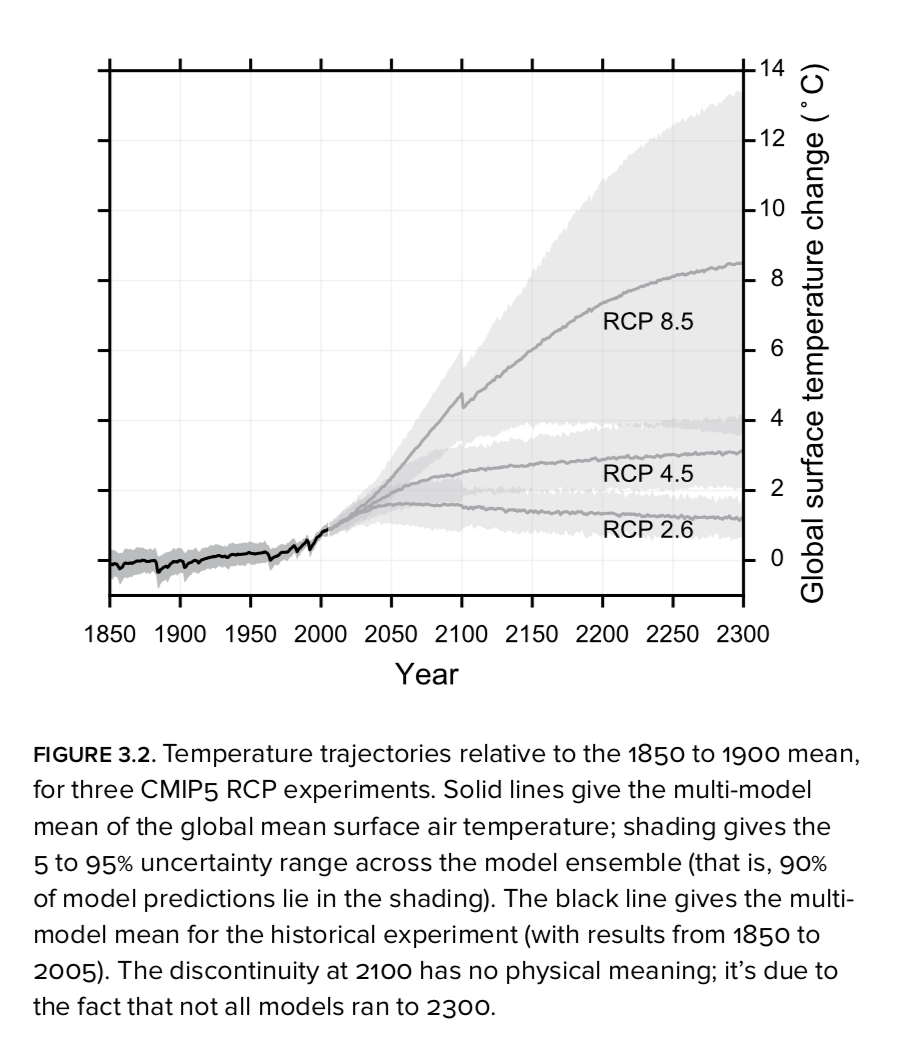
Temperature trajectories (with large uncertainties) for various representative concentration pathways (RCPs) from now to 2300 are shown in Figure 3.2.12 RCPs define future greenhouse gas concentrations under hypothetical emission scenarios. Scientists can then run global climate models with these predefined concentrations, facilitating comparison and collaboration. RCP 8.5 is the business- as-usual scenario, while the other two RCPs in Figure 3.2 represent varying levels of mitigation. The lower the RCP number, the more mitigation it presumes.13
In RCP 2.6, greenhouse gas emissions peak before 2020 and then decline rapidly, and warming stays below 2°C. However, this path- way is no longer achievable due to our collective procrastination.14
RCP 4.5 is a less aggressive pathway that’s still open to us. In it, models predict global mean surface warming of 2.4±0.5°C by 2100 over preindustrial levels (and 3.1±0.6°C by 2300).15
Our current trajectory is best approximated by RCP 8.5. If we choose this pathway, models predict mean surface warming of 4.3±0.7°C by 2100 (and 8.4±2.9°C by 2300). Note also that in RCP 8.5, warming accelerates rapidly in the 21st century: global temperature rises more during the second half of the century than during the first half.
To put these numbers in one context, the last glacial maximum, in which ice sheets covered not only Greenland but most of North America and much of northern Europe and Asia about 20,000 years ago, was 4.0±0.8°C cooler than in modern preindustrial times.16 To put them in another context, the last time the planet was about 2°C warmer was 125,000 years ago (the Eemian Maxi- mum, long before humans evolved),17 and it has been tens of mil- lions of years since the planet was 4°C to 8°C warmer.18
The distinction between social and scientific uncertainty is well-illustrated by Figure 3.2. The large spread covered by all the different RCPs indicates social uncertainty; physical science cannot predict what humans will do. On the other hand, the width of the shaded swath for each RCP gives a particular estimate of the scientific uncertainty: the spread between different models.19 This estimate, however, doesn’t capture uncertainty due to physical processes that aren’t modeled in the first place—the “unknown unknowns.” These could include various carbon cycle feedbacks, discussed below, which might augment warming.
Under all of the RCP scenarios, significant warming persists for many centuries, far beyond 2300, but the peak temperatures are very different. It’s unclear exactly what those peak tempera- tures will be or when they’ll occur because far-future model predictions become increasingly uncertain. But I think for our purposes here, and for the purposes of policymakers, Figure 3.2 provides a clear enough picture: to prevent warming far beyond levels humanity has ever experienced, we need to mitigate immediately and rapidly.
The physical basis for warming
Let’s now examine the causes of warming and how warming inter- acts with the Earth system. Along the way we’ll continue develop- ing our understanding of what we know and what we don’t know.
The Earth system
The Earth system is tremendously complex. Its main parts, viewed in the big picture and from the perspective of climate, are the at- mosphere, the ocean, the land, the ice, and the biosphere. They interact with one another via physical, chemical, and biological processes, over space scales ranging from microscopic to plane- tary, and time scales ranging from nearly instantaneous to billions of years.
Before I switched into atmospheric science, I studied neutron stars and black holes. Everything knowable about a stable isolated black hole is (we think) encoded in just three numbers: mass, elec- tric charge, and spin. But the state of the Earth depends on every cloud, tree, drop of moisture, mountain peak, ocean eddy, patch of snow, bacterium, and internal combustion engine. Instead of just three numbers, the state of the Earth system is described by an essentially infinite number of numbers. And to understand the system, we need to understand how they interact.
Despite this internal complexity, the Earth’s climate system interacts energetically with the universe in only three significant ways: by absorbing sunlight, by reflecting sunlight, and by emitting infrared light. Infrared light is invisible to humans, but we feel it as radiant heat when we sit near a fire. The key fact about infrared emission is that hotter objects emit more infrared energy than cooler objects. This fact allows the Earth system to balance the sunlight energy coming in with infrared energy going out to cold space. For example, if the sun became dimmer, the Earth would cool.
A cooler Earth would emit less infrared light, eventually arriving at a new balance at a cooler temperature.
The greenhouse effect
Greenhouse gases like CO2 act like a blanket warming the planet. We need this blanket. Without it the Earth’s average surface tem- perature would be −18°C (0°F) and there could be no life as we know it.20 So the greenhouse effect per se is not a bad thing. The problem is that by burning fossil fuels into the atmosphere we’re causing the blanket to become warmer. By 2014 we’d already in- creased the atmospheric CO2 fraction by 43% over preindustrial levels, and this increase is accelerating exponentially.21
Have you ever thought about how a blanket works? Imagine being naked without a blanket on a cool, windless night. Like any warm object, your body emits infrared radiation which carries away energy, cooling you off. Now imagine that you have a blanket. The underside of the blanket absorbs your emitted infrared energy, heats up, and then re-emits infrared radiation back to you. Some heat, however, is conducted through the blanket, causing the relatively cool top side to emit more infrared energy out into the air. But the top side of the blanket is cooler than your body, so it radiates less energy. This system reaches equilibrium when the top of the blanket loses infrared energy at the same rate that heat is conducted from its underside. The thicker the blanket, the less heat it conducts, and the hotter it gets underneath before reaching equilibrium.22
In place of body heat, the Earth’s main source of energy is in- coming sunlight. About 70% is absorbed, and the rest is reflected back into space by clouds, ice, snow, and other bright surfaces. Like your body on a cold night, the warm Earth loses heat by emitting infrared radiation into space. Greenhouse gases in the atmosphere act like the blanket, with a warm underside facing Earth (the lower atmosphere) and a colder top side facing space (the upper atmo- sphere). Greenhouse gases in the atmosphere absorb some of the infrared energy emitted by the Earth’s surface.23
The warmer lower atmosphere then radiates some of this infrared energy back down to the Earth’s surface. It radiates in the upward direction, as well; this radiation is trapped by the higher atmospheric layers, in turn (think of the atmosphere as many thin layers). The upward- directed infrared radiation from the cold upper layer streams into space, but since that highest layer is colder, it emits less energy than the planet’s surface.
What if we suddenly increase infrared-absorbing greenhouse gases? This makes the atmosphere act like a better blanket, and a smaller fraction of the upwelling surface infrared escapes into space. Because the absorbed solar energy hasn’t decreased,24 there is now an energy imbalance, and Earth warms. Warmer objects emit more infrared radiation, and eventually the escaping infrared energy will once again balance the incoming solar energy, despite the warmer blanket. Eventually the Earth will regain energy balance but at a warmer temperature.
Greenhouse gases
The main two human-emitted greenhouse gases are carbon diox- ide (CO2) and methane (CH4). Human emissions of halocarbons and nitrous oxide (N2O) also contribute, but to a lesser degree. Each gas is made from atoms electromagnetically connected in a particular geometric configuration. These geometries have specific resonant frequencies that determine how the gas interacts with infrared radiation.
The Earth system exchanges energy primarily by absorbing shortwave solar radiation and emitting longwave infrared radiation. We call factors that change one or the other of these two quantities radiative forcings. The Earth is in energy balance when the net radiative forcing is zero. Increasing the atmospheric con- centration of a greenhouse gas decreases the outgoing longwave radiation, and this change (in units of power per area, W/m2) is an example of a radiative forcing.
Water vapor (H2O) is the largest contributor to the green- house effect, but we humans have no direct control over it. It remains in dynamic equilibrium, evaporating into the atmosphere and condensing out as rain. A hotter atmosphere, though, holds more water than a cooler atmosphere. As we warm the atmosphere with the other greenhouse gases, water vapor acts as an amplifier. Ozone (O3) is another greenhouse gas which humans influence indirectly (via atmospheric chemistry).
Today human emissions do directly influence the atmospheric amounts of the other greenhouse gases. The global warming im- pact from emitting a tonne of some greenhouse gas depends on how efficiently that gas absorbs infrared light, as well as how long it stays in the atmosphere—its residence time.25
To allow for apples-to-apples comparisons of different green- house gases, we can integrate atmospheric absorption over the residence time of a gas species to calculate its global warming potential (GWP). GWPs are estimated relative to CO2, and given in units of “CO2-equivalents” (CO2e). For example, after 100 years, a tonne of methane causes a total of about 34 times more warming than a tonne of CO2; we say it has a GWP of 34 on a 100-year horizon, or GWP100 of 34. However, methane is reactive and has a residence time of only about 12 years, so on a 20-year horizon, its total warming potential relative to CO2 is even higher: the GWP20 of methane is about 105.26
The choice of time horizon is subjective, but important – especially for methane. Some methane inevitably escapes during natural gas extraction, processing, and distribution. Most analysts choose GWP100 over GWP20, downplaying the contribution of this leakage to global warming and making natural gas appear more attractive as a “bridge fuel.”
Nitrous oxide, N2O
Anthropogenic nitrous oxide in the atmosphere is produced mainly by the agricultural use of nitrogen fertilizers. It’s also produced by internal combustion engines and the breakdown of live-stock manure and urine. It resides in the atmosphere for 120 years, and has GWP20 of 260 (with a GWP100 that’s essentially the same due to a residence time of over 100 years).27 Human emissions of nitrous oxide accounted for about 5% of the current greenhouse radiative forcing (measured in 2011; see Figure 3.7, page 50, which we will discuss below).28
Halocarbons
Halocarbons are chemicals containing at least one carbon atom and halogen atom (usually chlorine or fluorine), useful as refrig- erants, solvents, pesticides, and electrical insulators. They were regulated in the 1990s because they deplete Earth’s protective stratospheric ozone layer (and also create dramatic “ozone holes” over the poles). Out of this family of compounds, the CFC-12 (CCl3F, brand name Freon-12, formerly common in refrigerators, Silly String, air horns, gas dusters, and other applications requir- ing an easily compressible gas) still has the most impact on the climate, with a residence time of about 100 years and a GWP20 of about 10,800.29 While emissions of CFC-12 have stopped, its global warming impact will continue for many decades. Mean- while, emissions of other halocarbon compounds are increasing. Human emissions of halocarbons account for another 5% of the greenhouse radiative forcing (see Figure 3.7, page 50).30
Methane, CH4
Methane is a powerful greenhouse gas (GWP20 of about 105,31 with an uncertainty of about 30%) with a short residence time of about 12 years. These two facts mean that mitigating methane emissions would have an immediate and significant impact on our warming trajectory.
Human emissions of methane account for about 30% of the current (instantaneous) greenhouse radiative forcing (see Figure 3.7, page 50).32 In terms of GWP (integrated over time), in 2010 it accounted for 16%33 or 37%34 of anthropogenic greenhouse gas emissions on a GWP100 basis or a GWP20 basis, respectively.
Over the last 200 years, atmospheric methane concentration has almost tripled, from 650 ppb (parts per billion) to 1,800 ppb.35
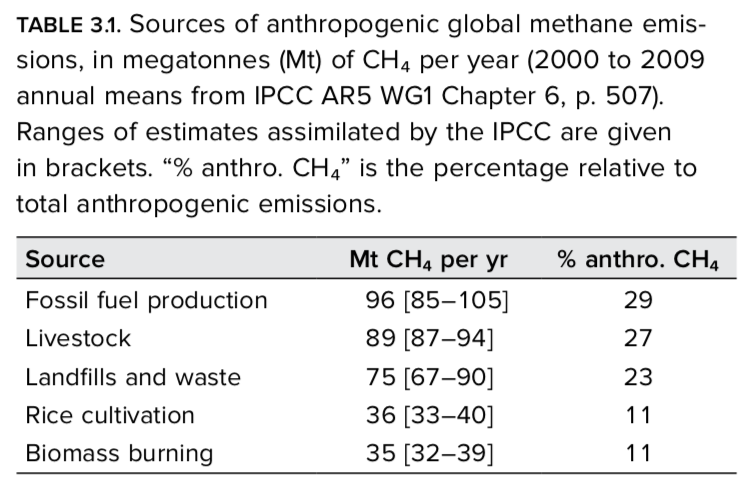
From 2000 to 2009, 50–65% of global methane emissions came from human activities; the remaining 35–50% came from natural sources, mainly from anaerobically decomposing matter in wet- lands. This source of methane may increase in the near future due to melting permafrost in northern regions, but the size of the in- crease is still highly uncertain.
Table 3.1 gives methane emission estimates from human activi- ties (annual means from 2000 to 2009). The largest anthropogenic sources of methane are fossil fuel production<sup>37</sup> (leakage) and livestock (75% of which is from cattle, who burp methane generated by fermentation in their digestive tracts). Each of these two sources accounts for between 4% and 10% of total anthropogenic greenhouse gas emissions, depending on choice of GWP time horizon.36
Carbon dioxide, CO2
CO2 is the principal driver of global warming. Human emissions of CO2 accounted for about half of the 2011 greenhouse gas radi- ative forcing (see Figure 3.7, page 50). When considered on the extended GWP100 basis instead of the instantaneous radiative forc- ing basis, however, CO2 accounts for three-quarters of warming, because it remains in the atmosphere for a very long time.
Humans cause CO2 emission by burning fossil fuels and re- moving forests. Approximately 90% of anthropogenic CO2 currently38 comes from burning fossil fuels, while approximately 10% comes from deforestation.39 The amount of CO2 released from removing forests is still uncertain, though, and current net CO2 emissions from deforestation could range from 1% to 20% (with fossil fuel burning taking up the remainder). In the past, deforestation played a larger role. One-third of net cumulative emissions from 1750 to today are due to land-use change (mainly deforesta- tion), which releases the carbon stored in wood and soils into the atmosphere via decomposition or fire.40
The residence of CO2 in the atmosphere is complex, medi- ated by multiple processes transferring carbon between the res- ervoirs—the atmosphere, the ocean, the biosphere, and the rocks—on different time scales. (We’ll discuss this “carbon cycle” in more detail below.) Because of this, the residence time of CO2 isn’t captured well by a single number. If humans stopped emit- ting CO2 today, in a few hundred years, one-quarter or so of what we’d emitted would remain in the atmosphere, and in a few tens of thousands of years, one-tenth or so would remain.
Atmospheric CO2 fraction has been precisely measured, to a small fraction of a part per million by volume (ppmv) high on Mauna Loa in Hawaii since 1958.41 Today, the CO2 fraction is measured at many different locations; as you’d expect, it tends to be a bit higher over areas of intense human activity. The annual high points in the Mauna Loa record are about two ppmv above the global average, Mauna Loa being in the northern hemisphere where 90% of humanity lives.
Atmospheric CO2 fraction from Mauna Loa and from the global average are shown in Figure 3.3.42 Notice the annual variation. The CO2 fraction increases during the northern hemisphere winter months (from October to May) and decreases during the summer months (from May to October). Most of the world’s plants are also in the northern hemisphere, and during the northern summer months, plants are actively growing and incorporating CO2 into their bodies. In the winter months, there is less growth but decomposition continues, releasing carbon back into the atmosphere via the tiny oxidative “fires” of biological respiration. Many have pointed out that this cyclical variation is like the biosphere breathing.
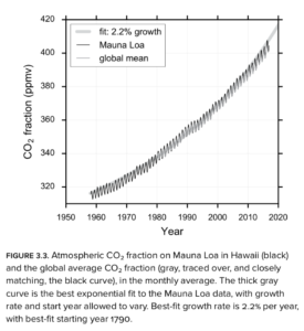
CO2 fraction in our atmosphere has risen exponentially; the best exponential fit (thick gray curve in Figure 3.3) has growth starting in 1790, increasing annually at a rate of 2.2%.43 In 1790, of course, James Watt had just succeeded in commercializing the steam engine. It’s remarkable that an atmospheric CO2 fraction record beginning in 1958 points back so precisely to humanity’s fossil fuel revolution.
What about further back in time? Figure 3.4 shows the CO2 fraction going back to 800,000 years ago from three ice cores in Antarctica, including a zoomed-in view of the last 12,000 years. Ancient air bubbles trapped in the ice are analyzed for their CO2 fraction, and time is inferred from the depth in the ice core.44

A few interesting things leap out of this record of nearly a mil- lion years of CO2 fraction. First, CO2 fraction is obviously much higher today than it has been at any time in the last 800,000 years. Second, the CO2 fraction was remarkably constant over the last 11,000 years, allowing for the stable climate which supported the rise of agriculture and complex civilizations. Third, during this epoch, there were a dozen or so relatively rapid and significant rises in CO2 fraction, although these were all far slower than the rise happening today, and stopped below 300 ppmv (whereas ours will clearly go far beyond 400 ppmv). For example, the rise beginning about 140,000 years ago took 10,000 years45 from be- ginning to end, and maxed out at about 290 ppmv. These rises correspond to transitions from glacial periods to interglacial periods. Fourth, the CO2 increases happened much more quickly than the CO2 decreases, giving a sawtooth pattern to the record. Although re-uptake of CO2 is complicated and controlled by multiple processes, this suggests that our current warming might last tens of thousands of years. We’ll see below that this is likely about right.
What human activities cause the most greenhouse gas emissions, worldwide? Estimates for 2010 are shown in Table 3.2.46 It’s striking how human emissions come from a multitude of sources; no single line item dominates the list. This reflects the deep penetration of fossil fuels into today’s predominantly industrial way of life.
What humans do: Sources of global warming
The estimate for the agriculture, forestry, and other land-use (AFOLU) sector has relatively high uncertainty, as it is difficult to separate natural from human-made emissions. Livestock production (which includes clearing of land, manure decomposition, feed production, and enteric fermentation) accounts for 10–20% of humanity’s global emissions.47 The transportation sector is grow- ing faster than any other, more than doubling between 1970 and 2010.48

Increasing global temperature
Figure 3.5 shows the average surface temperature of our planet since 1850, relative to the mean value of 1850–1900.49 These data originate from land weather stations and ocean surface temperature estimates from ships and buoys, which are statistically com- bined to produce a global average estimate.50 Care is taken to avoid biases from a variety of causes, such as imperfect sampling (you can’t put a thermometer on every meter of the Earth’s surface). However, despite this care they have been shown to be biased about 10% too low, if we interpret them as estimates of surface air temperature, as they use surface water temperature over the oceans.51 Therefore, although this data set estimates that 2015 was 1.1°C to 1.2°C warmer than the historical mean, the truth was likely between 1.2°C and 1.3°C. Similarly, 2016 was likely 1.4°C to 1.5°C warmer than the historical mean.


Ocean heat content provides an even better measure of global warming, albeit less immediate to the human experience. The oceans absorb 93% of the heat pouring into the planet due to the energy imbalance from human greenhouse gas emissions, and ocean heat content has less variability than surface air temperature.54 The global increase in ocean heat content since 1955, in the ocean layer from the surface down to a depth of 2,000 meters, is shown in Figure 3.6.55
Today’s global warming is occurring more rapidly than any known warming in Earth’s geologic history by more than a factor of ten.56 Unsurprisingly, our planet is changing radically as a result. The rate of Greenland ice sheet loss has increased from 34 giga- tonnes (Gt) per year from 1992–2001 to 215 Gt per year from 2002– 2011, a staggering six-fold increase in just a decade;57 the ice sheet is lowering by 1.5 m per year around its edges.58 Sea level has risen by about 20 cm and is rising at about 1/3 of a centimeter per year,59 and accelerating.60
The Arctic sea ice is roughly half gone (as of 2014, measured by summer minimum ice extent) and vanishing rapidly: summer ice extent is decreasing at a rate of between 9% and 14% per decade.61 And, of course, hot days and heat waves are increasing in frequency and severity.62 All of these changes are further evidence of warming, independent “thermometers.” The Earth’s warming is unequivocal, and the impacts are accelerating.63
But the climate system, of course, interacts complexly with the rest of the Earth system and is highly variable. Even as the global surface temperature increases, regional and temporal variations can create local or temporary colder weather. Indeed, changes in air and ocean circulation patterns caused by global warming could conceivably lead to regional cold anomalies. It’s also quite possible for heat to be transferred from one part of the climate system to another, for example from the surface to ocean sublayers. It’s important to remember that our ability to monitor the climate system is limited, and that particular variables (such as surface air temperature) impose their own idiosyncrasies and limitations on our view of the system.
The drivers of global warming
Radiative forcing estimates allow us to rank different drivers of global warming such as atmospheric CO2, or changes in the sun’s radiance. Figure 3.7 summarizes the state of our knowledge.64
It’s worth carefully unpacking this figure, which gives radiative forcings in 2011 relative to 1750. First, note that 98% of the total change in forcing is human-caused. Most of this is due to human- emitted gases. The forcing from solar changes since 1750 are minis- cule compared to human-caused changes; and over the last few decades, the sun has, in fact, been getting cooler.65 In other words, relative to a few decades ago (as opposed to 1750), more than 100% of the forcing is attributable to humans.
Albedo changes due to land use (albedo means reflectivity) are from human-caused changes to the land surface, such as cutting down dark forests and replacing them with brighter crops and cities, which reflect more sunlight. These changes have a net cool- ing effect, and so are a negative radiative forcing. However, land- use change also causes CO2 emissions, a positive forcing.
For each emitted compound, the figure includes indirect contributions from processes caused by the emission. For example, consider methane, CH4. In addition to its direct greenhouse gas forcing, methane induces the creation of ozone (O3) and strato- spheric (high-altitude) water (H2Ostr), then eventually oxidizes to become CO2. (As in the figure, I’ve listed these effects from strongest to weakest. Note that the shading in the figure’s bars correspond to the “resulting drivers” as listed.) Ozone, water, and CO2 are also greenhouse gases. If we tallied these indirect effects somewhere else, we would underestimate the climate impact of human methane emissions. Halocarbons, on the other hand, destroy ozone, creating an ozone hole and producing a negative (cooling) forcing. Tallying this elsewhere would lead us to over- estimate the effect of halocarbons.66
Note that human emissions of CO and NOx don’t contribute directly to the greenhouse gas forcing
they aren’t greenhouse gases—but they do contribute indirectly via atmospheric chemis- try (the creation and destruction of gases like CH4, O3, and CO2).
Next, note that some aerosol pollution—especially sulfates and organic carbon from burning biomass—counteracts warming. These aerosol particles in the air reflect sunlight like tiny mirrors. I’ve referred to this group of aerosols as “bright aerosols” in the figure. They also act as cloud condensation nuclei, brightening clouds by inducing smaller but more numerous water droplets and increasing the cloud cover. These effects are “cloud changes due to aerosols.”
You may have noticed the prominent plateau in warming between 1940 and 1978 in Figure 3.5; this is likely due to an increase in bright aerosol pollution.67 Ironically, if we somehow suddenly eliminated these pollutants, the global warming forcing could con- ceivably jump up by almost 40%, although the uncertainty here is still quite large.
Black carbon, on the other hand, contributes significantly to warming. Black carbon is an aerosol produced in the agricultural burning of forests and savannas, residential biomass burning, and diesel engines. Instead of reflecting sunlight, black carbon absorbs it, giving a positive forcing of similar magnitude to methane’s direct greenhouse gas effect.68
Finally, the figure gives the trend in total anthropogenic radiative forcing, from 1950 to 2011. We humans have nearly doubled our global warming impact since 1980. Radiative forcing is accelerating rapidly, driven mainly by exponentially increasing CO2 emissions.

Radiative forcings are half of the story. We’re now ready to dis- cuss the other half: how the Earth system changes as a result of these forcings.
Earth system feedbacks
Increasing greenhouse gas concentrations in the atmosphere force the Earth to a warmer state. Meanwhile, the Earth system changes in response to this forcing. The total amount of warming for a given greenhouse gas concentration—the climate sensitivity— depends on how the Earth responds to the forcing.
Increasing greenhouse gas concentrations in the atmosphere force the Earth to a warmer state. Meanwhile, the Earth system changes in response to this forcing. The total amount of warming for a given greenhouse gas concentration—the climate sensitivity— depends on how the Earth responds to the forcing.
Processes that further enhance warming are called positive feed- backs (positive as in they go in the same direction as warming, not as in good), while processes that slow warming are called negative feedbacks. Together, forcings and feedbacks determine the temperature.
I’ve already mentioned a fundamental positive feedback: a warmer atmosphere holds more water vapor, which is a strong greenhouse gas. I’ve also mentioned a fundamental negative feed- back: hotter objects lose more heat through infrared emission. Here are two other important feedbacks:
- Surface albedo: I’ve already mentioned albedo in the context of land-use change: when forests are destroyed and replaced with agriculture or human development, more sunlight is reflected to space (albedo increases). On the other hand, ice and snow reflect more sunlight than the ocean or soil exposed after it melts. This is a positive feedback: as ice and snow melt, the surface absorbs more sunlight, warming further. Albedo feedback due to sea ice loss is an important driver for changes occurring in the Arctic, which is warming more rapidly than the rest of the planet—and more rapidly than scientists expected.69 Snow and ice albedo is also lowered by algae growth and buildup of anthropogenic soot.
- Clouds: Small changes in the global cloud cover can have large repercussions on climate. Clouds can block incoming sunlight (playing a huge role in global albedo) as well as outgoing infra- red light; different kinds of clouds have different effects. Low- altitude clouds like cumulus (puffballs) and stratocumulus (overcast clouds) are warm and thick. They reflect sunlight, but because they’re nearly as warm as the surface, they don’t have a strong effect on the net upwelling infrared radiation; their net effect is cooling. Cold, wispy high-altitude clouds let sunlight through, but they absorb upwelling infrared light. Since these high cloud tops are cold, they don’t emit much infrared. So their net effect is warming. The overall cloud feedback is likely positive: cloud changes are amplifying global warming.70
Surface albedo and clouds both contribute to Earth’s global planetary albedo, which has a value of 0.29; Earth reflects a bit less than a third of the total incoming sunlight back into space. Global planetary albedo represents an average of all the ice, clouds, water, forests, cities, and deserts. Globally, clouds seem to act as a stabilizing buffer to the planetary albedo system in ways that we don’t yet fully understand.71
There are additional climate feedbacks associated with the carbon cycle.
The Earth’s carbon cycle
Carbon gets cycled through the atmosphere, the ocean, geological formations, and the bodies of all living things. Over the last four billion years of Earth’s history, the processes of the carbon cycle have acted like a thermostat, tending to maintain a climate with liquid oceans, even when the sun was fainter in its youth.
This stability has allowed Earth’s biodiversity to flourish.
On shorter time scales, however, the carbon cycle amplifies abrupt cli- mate changes; these climate changes played an important role in the bio- sphere’s previous mass extinctions.2 These past examples of carbon cycle amplification inform our current global warming event.
There are several major reservoirs of carbon on Earth that vary widely in size and interact with each other and with the climate system on vastly different time scales; see Table 3.3.73 Before the industrial era, carbon flows between these reservoirs were roughly in balance—no net flows. Now, because of human emissions, there are imbalances and net flows. The CO2 we emit accumulates in the atmosphere, but also spills into other reservoirs on various time scales. Currently about 57% of the CO2 we emit does not end up in the atmosphere;74 instead, it’s absorbed by the ocean, biomass, and soils, all of which are acting as “carbon sinks.” In general, these carbon sinks are poorly understood; but it seems likely that over the next few decades or centuries they’ll decrease in effectiveness, as the ocean becomes increasingly saturated and the land reservoirs respond to a warmer world.75

- The atmosphere: While small in size, this key reservoir inter- connects many parts of the carbon system, a Grand Central Station of the carbon cycle. Carbon flows in from the ocean, the respiring biosphere, and from burning fossil fuels and forests; and carbon flows out into the ocean and into the grow- ing biosphere (mainly trees). Because of additional emissions from humans, in the 2000s carbon was accumulating in the atmosphere at an average rate of 4.0±0.2 GtC (gigatonnes of carbon) per year.76 This accumulation rate is likely to increase due to our accelerating emissions, and also due to a slowdown in uptake from the ocean and land reservoirs.
- The ocean: About 28% of the total CO2 we’ve emitted so far has been absorbed by the ocean and converted into carbonic acid.77 As the ocean warms and becomes increasingly saturated with CO2 it will become a less efficient sink. This means more of our emitted CO2 will remain in the atmosphere, accelerating warming. There is some evidence that the ocean carbon sink is already becoming saturated,78 but our understanding of how the ocean sink works and how it will work in the future remains uncertain. Indeed, we know (from isotopic analysis) that the ice age cycle was driven by a positive feedback loop involving ocean uptake of CO2. During glacial times, the colder ocean some- how pulled more CO2 out of the atmosphere than can be explained by the temperature dependence described above. However, we don’t know what additional process (or processes) were operating. We can’t eliminate the possibility that this additional unknown feedback might also operate in re- verse, contributing to warming.79
- The land: Soil and plants (which are intimately intercon- nected), together with permafrost, make up the land carbon reservoir. Increased atmospheric CO2 augments plant growth and therefore plant carbon uptake, up to a point.80 We don’t know how to directly measure the size of this land carbon sink, but we infer that, on average, about 29% of the total CO2 we’ve emitted has been absorbed by the land sink (that is, the total sink, 57%, minus the ocean sink, 28%). Annual variability of land carbon uptake is high. During some El Nino years, the land “sink” ends up being a net source; in other years, it ab- sorbs more than 29%. It’s still unknown where and how this absorbed carbon is apportioned between tropical forests and boreal forests. Unfortunately, however, there’s strong empirical evidence that future warming will drive a net loss of soil carbon to the atmosphere,81 and that global forest mortality and wild- fires will increase in the future—and that these sources of atmospheric carbon have been underrepresented in projections to date.82 We might see the catastrophic loss of the Amazon rain forest and release of its carbon into the atmosphere within decades, as drought makes the forest increasingly susceptible to fire,83 and projected severe drying in the 21st century pushes it toward a tipping point.84 About a quarter of the northern hemisphere is covered in permafrost. As the permafrost thaws, microbes convert the biomass (mostly peat) into CO2 if oxygen is present, and CH4 if oxygen isn’t present. It’s estimated that there are about 1,700 GtC in the permafrost, more than four times what we’ve emitted from burning fossil fuels. The rates of permafrost CO2 and methane release as the planet warms are unknown. It’s likely that the global land carbon sink will switch from being a net carbon sink to a net carbon source, accelerating cli- mate change. However, as with our understanding of the ocean sink’s future, uncertainty about the details is high.85
- Frozen ocean methane: Methane is frozen in ocean sediments on continental shelves. There’s a lot of it, thousands of GtC worth, many times the carbon that humanity has so far emit- ted. If the Earth warmed enough to begin releasing this methane, it would be a positive feedback. Everything about ocean methane release is uncertain—mechanism, magnitude, and timing—but we might be wise to plan for at least 0.5°C additional warming from ocean methane release after 3°C of global warming, and this warming boost could last for thousands of years.86 Most climate models don’t yet include the carbon- thawing feedbacks (permafrost and frozen ocean methane), biasing their predictions of future warming toward being too conservative. Slow release from these reservoirs could ultimately end up contributing about the same amount of CO2 to the atmosphere as humans end up emitting, effectively doubling our emissions; exactly how this plays out, though, is anyone’s guess.87
- Limestones: Carbonate rock (limestone) is the largest carbon reservoir, and it interacts with the climate system on tectonic time scales, as we’ll discuss below.
- Fossil fuels: Humanity had burned a total of 375±30 GtC of fossil fuels as of 2011, and in one year (2011), we burned 9.2 GtC.88 Between 2000 and 2010, our global greenhouse gas emissions accelerated exponentially at 2.2% per year;89 this in- crease was driven by an increase in our burn rate. (Recall that the measured atmospheric CO2 fraction has this same growth rate over the long term; see Figure 3.3, page 42.)
- Kerogens: When organisms die on land or in the ocean, their carbon can become trapped in kerogens—fossil fuel precursors—which can eventually transform into coal, oil, and natural gas. As with the rock sink processes, these processes operate on long time scales. Both the rock and the kerogen sinks will be irrelevant on human time scales, but over millions of years, they will be significant. Perhaps in ten or 100 million years, Earth’s “battery” will once again be charged, with much of the fossil carbon that humans dug up and burned again buried underground in the form of coal, oil, and gas.

This weathering cycle is an important part of the Earth’s thermostat system. In the distant past, almost a billion years ago, there may have been a period when the planet was a frozen “snowball Earth.” Volcanic emission of CO2 and reduced rock weathering are thought to have helped bring the Earth out of this period. This flow is significant on time scales of hundreds of thousands of years.
Another flow, not as slow, involves the ocean floor sediments which contain accumulated calcium carbonate shells. CO2 dis- solves in the ocean by combining with carbonate ions to make car- bonic acid, which dissociates into bicarbonate.91 This makes the water more acidic, which then dissolves the sediments,92 releasing more carbonate ions which are then available to react with CO2. The ocean floor sediment buffer therefore allows the ocean to dis- solve more CO2 than it otherwise would. There’s a catch though: we’ll need to wait thousands of years for this exchange to help us, as the time scale for the acidic surface waters to reach the sediments is set by the time scale for deep ocean water mixing. We’ll discuss the lingering fate of our CO2 emissions in the next chapter.
Summary: The cause of global warming
Multiple lines of evidence show that humans are causing the ob- served exponential increase in atmospheric CO2. For example, we know roughly how much CO2 we emit each year from burning fossil fuels because the fossil fuel industry keeps track.93 We also know that about one-third of our total emissions have been from deforestation. We can thus directly compare an estimate of our accumulating CO2 emissions to what we see in the atmosphere.94 To account for deforestation, I’ve multiplied the fossil fuel data by a factor of 1.3 and plotted this as a dotted black line in Figure 3.8, alongside the actual observations from Mauna Loa (gray line; we discussed these observations above).95
That dotted black line shows that since 1965 humans have emitted about twice the CO2 that remains in the atmosphere. As discussed earlier, we know that 28% goes into the ocean, and the rest (29%) must be going into the land because there’s no other plausible place for it to go. The solid black line accounts for these carbon sinks, in good agreement with observations. This provides unequivocal evidence that humans are the cause of the observed CO2 increase.
In case that’s not enough, here are four additional lines of evi- dence: 1) decreasing atmospheric oxygen is consistent with what we’d expect from a fossil fuel source; 2) the downward trend over time of the 13C/12C isotopic ratio is consistent with what we’d expect from a fossil fuel source; 3) the downward trend over time of the 14C/12C radiocarbon isotopic ratio is consistent with what we’d expect from fossil fuel and nuclear testing sources; 4) the difference in atmospheric CO2 concentration measured in the northern and southern hemispheres, and the increasing trend in this difference over time, are both consistent with what we’d ex- pect from a fossil fuel source.96


A second line of evidence comes from the ice core samples. We’ve already seen that, by analyzing trapped bubbles of ancient atmosphere, we can directly measure the atmospheric CO2 fraction back to 800,000 years ago; we can also infer the Antarctic surface temperature record from water isotopes.98 Figure 3.999 shows a strikingly clear correlation between temperature and atmospheric CO2 fraction. Correlation doesn’t imply causation, and in fact the ice core CO2 changes lag the temperature changes and are thought to be amplifiers instead of initial drivers;100 but the correlation certainly does mean that a present-day lack of warm- ing, given the observed human-caused CO2 spike, would require explanation. CO2 initiating warming might be unique to today’s ongoing climate change.101
The third link comes from models. As we’ve seen, there are many factors controlling the global temperature in addition to the CO2 fraction. For one thing, other human-emitted greenhouse gases add to the warming, and human-emitted aerosol pollutants reflect sunlight and block some of the warming. There are clouds and other Earth system feedbacks, there are multiple carbon sinks and natural carbon sources, there are small changes in the sun’s in- tensity, and there are even volcanoes sporadically emitting cooling aerosols. Earth system models attempt to account for as many of these complex and interacting processes as they can. Of course, their predictions differ, as we explicitly saw in Figure 3.2, page 33, but every Earth system model says that increasing the CO2 fraction leads to warming.
In fact, no Earth system model is able to replicate the observed warming in the absence of rising CO2, and there’s no alternative explanation for the warming that’s consistent with observations. It’s my opinion, therefore, that any reasonable person must accept that human-emitted CO2 is a significant cause of the observed global warming—unless equally strong evidence to the contrary comes in. So far, I know of no such evidence.
- You can download the AR5: Intergovernmental Panel on Climate Change. “Assessment Reports.” [online]. ipcc.ch/publications_and _data/publications_and_data_reports.shtml#1. The panel is divided into three working groups. Working Group I (WG1) presents the physical evidence for global warming and resulting changes occurring in the Earth system. Working Group II (WG2) presents the current and future impacts and human adaptation strategies. Working Group III (WG3) presents our understanding of the scientific, technological, environmental, economic, and social aspects of climate change mitigation and quantifies mitigation pathways, e.g., how much warming will occur under various paths available to humanity. WG1 assesses and summarizes the scientific literature, whereas WG2 and WG3 summarize the scientific and socioeconomic literature. Each working group provides a 30-page Summary for Policymakers (SPM). Subsequent citations use these abbreviations to identify sections within this report.
- Here are some suggestions for further reading in order of increasing level of reader commitment. (1) Yoram Bauman and Grady Klein. The Cartoon Introduction to Climate Change. Island Press, 2014. (2) The 36-page overview US National Academy of Sciences and Royal Society. Climate Change: Evidence and Causes. National Acad- emies Press, 2014. [online]. ap.edu/catalog/18730/climate-change -evidence-and-causes. (3) David Archer. Global Warming: Under- standing the Forecast, 2nd ed. Wiley, 2011 (a college text for non- science majors). (4) “The Princeton Primers in Climate,” a series of definitive but accessible books focusing on subtopics of climate, each by an expert in the subtopic: Princeton University Press. Catalogue Primers in Climate. [online]. press.princeton.edu/catalogs/series /princeton-primers-in-climate.html. I’d advise against trying to learn about climate science solely from the internet, as you’ll have to wade through a great deal of misinformation and disjointedness. That said, you can find accurate (if disjointed) information at skepticalscience .com and realclimate.com.
- Many scientists and humanists have given this new epoch a strati- graphic name, the Anthropocene. I hesitate to follow them for three reasons. First, the word has been embraced by “ecomodernists” and others who believe, with a blind faith, that technology is the way out of our predicament. (I disagree.) Second, it makes our destructive presence feel like a geologic fact, thereby potentially reducing politi- cal will to do what we can to reduce human impact on the biosphere. Humanity still very much gets to choose just how bad global warming will get. Third, and perhaps most importantly, it presupposes that humans are the problem. In my opinion, humans aren’t the problem. A particular human culture is the problem.
- I surveyed my Earth scientist colleagues (participating in the survey required authorship on a peer-reviewed journal paper in Earth sci- ence) and received 66 responses. When asked “How often do you feel grief about global warming,” only 10% responded “never” (a one on a scale from one to five) while half of respondents feel significant grief (with 14% and 35% choosing five and four on the scale, respectively).
- IPCC AR5 WG1 SPM puts this temperature increase at 0.85°C, but this has since been revised upward by 24%: Mark Richardson et al. “Reconciled climate response estimates from climate models and the energy budget of Earth.” Nature Climate Change 6 (2016). [online]. doi:10.1038/nclimate3066. Temperature will increase to about 1.2°C by 2020 (2015 was already 1.1°C to 1.3°C above the pre-industrial baseline, but this was just a single year), and 1.4°C by 2030. These projections are linear extrapolations based on the observed warming of 0.12°C per decade between 1951 and 2012.
- Camilo Mora et al. “The projected timing of climate departure from recent variability.” Nature 502 (2013). doi:10.1038/nature12540.
Models are tools for predicting how variables might change in the future. A global climate model is software code that runs on supercomputers and represents physical, chemical, and biological processes in the atmosphere, ocean, land, and ice. Earth system models are global climate models that explicitly model the carbon cycle. These models represent the Earth by dividing it into three- dimensional grid cells; horizontal resolution is typically about 100 km, although this is falling as computers get faster. At each time step, variables in every grid cell (such as temperatures, cloud amounts, sea ice amounts, etc.) are updated based on values from the previous time step and values from neighboring grid cells.
- The business-as-usual scenario, named “RCP 8.5,” was described in Keywan Riahi et al. “RCP 8.5: A scenario of comparatively high greenhouse gas emissions.” Climatic Change 109(1–2) (2011). [on- line]. doi:10.1007/s10584-011-0149-y. The mitigation scenario, named “RCP 4.5,” is described in Allison M. Thomson et al. “RCP 4.5:
A pathway for stabilization of radiative forcing by 2100.” Climatic Change 109(1–2) (2011). [online]. doi:10.1007/s10584-011-0151-4.
These results used a model experiment called “historicalNat” to produce estimates of the range of background variability. In the historicalNat experiment, the models ran from 1860 to 2005 with no anthropogenic CO2 emissions, allowing for a pure comparison with the two RCP runs. However, only 17 climate models actually ran his- toricalNat, whereas 39 models ran an experiment called “historical” which included observed changes in atmospheric composition, in- cluding anthropogenic CO2 emissions. Mora et al. also report results using the historical experiment as the background variability. Because this already includes some warming, the climate departure dates relative to it are delayed relative to the historicalNat results, to 2047 for RCP 8.5 (this is a mean of the 39 models, with a standard error of three years) and 2069 for RCP 4.5 (with a standard error of four years). However, these results are clearly biased due to the anthropo- genic warming in the background. The results from the historicalNat do not have this bias. Mora et al. chose to highlight the biased results in order to be more conservative; in my opinion, this was a mistake. In science, it’s always best to report whatever is closest to the truth, to the best of your knowledge.
Note that surface temperature is just one variable in the Earth sys- tem. Any variable can be analyzed for anthropogenic departure. For example, global departure has already occurred for ocean surface acidity from anthropogenic CO2 dissolved in the ocean.
I therefore suggest we mitigate as if our lives depend on it. I person- ally don’t think there’s anything more important for humanity to do at this time.
Thanks to Jan Sedlacek for providing the underlying multi-model mean data, from which I created this black-and-white version of Figure 12.5 from IPCC AR5 WG1 (a.k.a. Matthew Collins et al. “Long-term Climate Change: Projections, Commitments and Irreversibility” in T. F. Stocker et al., eds. Climate Change 2013: The Physical Science Basis. Working Group I Contribution to the Fifth Assessment Report of the Intergovernmental Panel on Climate Change. Cambridge University Press, 2013, p. 1039).
The number gives the approximate radiative forcing in watts per square meter (W/m2) in the year 2100 for the scenario. We’ll discuss radiative forcing in detail later in this chapter.
Jasper van Vliet et al. “Meeting radiative forcing targets under delayed participation.” Energy Economics 31 (2009). [online]. doi:10.1016/j .eneco.2009.06.010.
See IPCC AR5 WG3 Chapter 12, Table 12.2. Predictions are the multi- model means. Uncertainties are one standard deviation of the multi- model distribution. Note that emissions predictions beyond 2100 require extended RCP scenarios, which make simple (and possibly simplistic) assumptions about greenhouse gas and aerosol emissions beyond 2100. As model predictions extend further into the future, they naturally become increasingly uncertain.
J. D. Annan and J. C. Hargreaves, J. C. “A new global reconstruction of temperature changes at the Last Glacial Maximum.” Climate of the Past 9 (2013). [online]. doi: 10.5194/cp-9-367-2013.
Lorraine E. Lisiecki and Maureen E. Raymo. “A Pliocene-Pleistocene stack of 57 globally distributed benthic δ18O records.” Paleoceanology 20(1) (2005). [online]. doi:10.1029/2004PA001071.
James Hansen et al. “Climate sensitivity, sea level and atmospheric carbon dioxide.” Philosophical Transactions of the Royal Society A 371 (2013). [online]. doi:10.1098/rsta.2012.0294.
A key reason the swaths in Figure 3.2 are so wide is due to a “known unknown,” our uncertainty about how clouds work. (One of my research interests is low-altitude clouds: how they interact with the Earth system, how they change as the planet warms, and how their changes in turn affect warming.) The global models used to make climate projections divide the Earth into grid cells that are currently about a degree latitude and a degree longitude in size—much larger than individual clouds. This means the models must statistically approximate cloud variables, such as the total cloud cover at different altitudes, in each grid cell. Each model does this differently, and one result of this is that the models differ on how clouds interact with at- mospheric dynamics, and how they’ll change as the planet continues to warm. For example, some models predict an increase in low clouds with warming, while others predict a decrease. Low clouds (such
as the stratocumulus clouds on an overcast day) cool the planet by reflecting sunlight back to space: models with more low clouds tend to predict cooler temperatures, and models with fewer low clouds predict warmer temperatures.
This temperature would be set by a simple balance between absorbed solar radiation and emitted thermal infrared radiation. There would not even be clouds reflecting sunlight and interacting with outgoing infrared light, because water vapor is among the greenhouse gases we’ve just imagined away. The Earth’s actual average surface tempera- ture, with the greenhouse effect, is about 15°C.
Inferred from data from NOAA Earth System Research Laboratory. “Trends in Atmospheric Carbon Dioxide.” [online]. esrl.noaa.gov /gmd/ccgg/trends/global.html.
The rate of heat conduction between two sides of a conducting object (like our blanket) is proportional to the difference in temperature between them.
This absorption is quantum-mechanical. Infrared photons coming
up from the Earth have a range of frequencies following the Planck spectrum. When an infrared photon hits a molecule of water or CO2 (or another greenhouse gas) with the quantum of energy needed to excite the molecule from its ground state to e.g., a bending vibrational state (i.e., molecules can only absorb photons of certain frequencies, but the photon happens to have one of these quantum-mechanically allowed frequencies), it can be absorbed by the molecule, which then starts to vibrate. After some time, the molecule will de-excite and emit a photon in a random direction, possibly out to space. However, in the lower atmosphere, the molecule is more likely to collide with some other molecule first. When this collision occurs, it can transfer energy to the molecule it collides with. The net result is that most of the upwelling infrared photons from the Earth’s surface fail to escape into space, and instead warm up the lower atmosphere.Measuring the global mean reflected solar energy from space is chal- lenging; satellites records show no clear trend. While you might think melting snow and ice would cause more solar energy to be absorbed (and this does happen regionally), cloud patterns can change and compensate in the global mean.
The residence time is an estimate of how long it would take for the excess over preindustrial levels to be halved. This doesn’t mean the next halving will take the same amount of time (i.e., the decay is not necessarily a single exponential process). CO2 is chemically inert and has a long residence time, while CH4 is chemically reactive and has a short residence time.
These values are from Drew T. Shindell et al. “Improved attribution of climate forcing to emissions.” Science 326 (2009), at p. 716. [online]. doi:10.1126/science.1174760. For a given gas, GWP estimates depend on which direct and indirect warming effects from that gas are in- cluded in the estimate. For example, the IPCC GWP estimates for methane do not include gas-aerosol interactions, in which methane suppresses the formation of aerosols which cool the climate; exclud- ing this effect, the IPCC AR5 estimates GWP20 of only 86.
PCC AR5 WG1 Chapter 8, p. 714 gives a GWP20 of 264 and a GWP100 of 265 with uncertainties 20% and 30% respectively.
Estimates of percentage of current greenhouse radiative forcing in this section are made by dividing the forcing in question by the total posi- tive forcing from greenhouse gases: CO2 + CH4 + halocarbons + N2O + CO + NMVOC = 3.33 W/m2. Note that I’ve omitted NMVOC from the discussion for simplicity (they contribute 0.1 [0.05 to 0.15] W/m2 and are declining); for details see IPCC AR5 WG1 Chapter 2.
IPCC AR5 WG1 Chapter 8, p. 731.
This 5% factors in the cooling effect of ozone destruction.
Shindell et al. “Improved attribution of climate forcing to emissions.”
This includes formation of ozone and stratospheric water vapor, but not gas-aerosol interactions.
IPCC AR5 WG3 SPM.
From my own calculation using a methane GWP of 105, based on the 16% figure for a methane GWP of 34, with the other greenhouse gas GWPs fixed.
IPCC AR5 WG1 Chapter 2, p. 167.
IPCC AR5 WG1 Chapter 6, p. 541.
Note that the IPCC estimate of methane emissions from fossil fuel production relies on a 2012 EPA estimate: US EPA, Office of Atmo- spheric Programs. “Global anthropogenic non-CO2 greenhouse gas emissions: 1990–2030.” EPA Report # EPA 430-R-12-006. [online]. epa.gov/climatechange/Downloads/EPAactivities/EPA_Global _NonCO2_Projections_Dec2012.pdf. Newer studies are finding that this estimate may be significantly too low.
- The 2002 to 2011 annual average.
- IPCC AR5 WG1 SPM. Between 2002 and 2011, on average humans emitted 8.3 [7.6–9.0] gigatonnes of carbon (GtC) per year from burning fossil fuels and making cement, and 0.9 [0.1–1.7] GtC per year from land-use change. Cement production accounts for about 4% of human CO2 emissions: IPCC AR5 WG1 Chapter 6, p. 489.
- IPCC AR5 WG1 Chapter 6, p. 486.
- The measurement process is described on the website of the Carbon Cycle Greenhouse Gases Group of the Global Monitoring Division of the Earth System Research Laboratory of the National Oceanic and Atmospheric Administration (online at esrl.noaa.gov/gmd/ccgg/). In a nutshell: Scientists at the top of the mountain measure the CO2 fraction in dried air via infrared absorption. Infrared light shines into a glass tube containing air. An infrared detector on the far side of the tube measures the transmitted infrared light. CO2 blocks infrared light (which is also why it warms the Earth), so the more CO2 in the air, the less infrared light makes it to the detector. The output of the detector is a voltage which increases with the power of the incident infrared radiation. Once calibrated, that voltage can be converted to the CO2 fraction to within 0.2 ppmv (parts per million by volume). The trickiest part of the measurement is calibration: accurately and precisely converting the detector voltage to the fraction of CO2 in the air. This is done with three reference mixtures of air, themselves carefully calibrated, which are turned on once per hour for four minutes each. The three data points are fitted quadratically, giving the conversion function. Systematic errors are guarded against by checking prepared “target” samples of air of various and known CO2 fractions, and by sending flasks of air to National Institute of Stan- dards and Technology (NIST) in Boulder, Colorado, for indepen- dent measurement.
- Data are from US NOAA. “A Global Network for Measurements of Greenhouse Gases in the Atmosphere.” [online]. esrl.noaa.gov/gmd /ccgg/. t-b
- I used the function y=280+(1+a) . The best fit values (on annual mean values from 1959 to 2016) are b = 1790 and a = 0.0217.
- The record going back to about 400,000 years ago comes from an ice core taken near Vostok Station, Antarctica: J.R.Petitetal.“Climate and atmospheric history of the past 420,000 years from the Vostok Ice Core, Antarctica.” Nature 399 (1999). [online]. doi:10.1038/20859. The CO2 fraction was measured by gas chromatography. Because
this is a “proxy” record, it has error bars in both axes (time and CO2 fraction). The error bar in the absolute time (the x-axis) is less than ±15 ky (kiloyears) over the whole record, and less than ±5 ky over the last 110,000 years. The error bar in the CO2 fraction (the y-axis) is ±3 ppmv. The record going back to about 800,000 years ago comes from an ice core taken on Dome C, Antarctica: Lüthi et al. “High- resolution carbon dioxide concentration record 650,000–800,000 years before present.” Nature 453 (2008). [online]. doi:10.1038 /nature06949. The record from 1,000 years ago until almost the pres- ent day comes from an Antarctic ice core taken on the Law Dome: Etheridge et al. “Natural and anthropogenic changes in atmospheric CO2 over the last 1000 years from air in Antarctic ice and firn.” Journal of Geophysical Research 101 (1996). [online]. doi:10.1029/95JD03410. - Although the error in absolute time at this point in the record is around ±5 ky, the error in time durations is much smaller.
- Data from IPCC AR5 WG3, Chapters 7–11. Note that this table pre- serves the GWP100 basis used by the IPCC. In other words, methane is assigned the relatively low GWP of 21, arguably making it under- represented in this table.
- M. MacLeod et al. Greenhouse gas emissions from pig and chicken supply chains—A global life cycle assessment. Food and Agriculture Organization of the United Nations (FAO), 2013. [online]. fao.org /docrep/018/i3460e/i3460e.pdf; C. Opio et al. Greenhouse gas emis- sions from ruminant supply chains: A global life cycle assessment. Food and Agriculture Organization of the United Nations (FAO), 2013. [online]. fao.org/docrep/018/i3461e/i3461e.pdf
- IPCC AR5 WG3 Chapter 8, p. 605.
- The data are from the Berkeley Earth. Land + Ocean surface temperature time series: Berkley Earth. Land + Ocean Data. [online]. berkeleyearth.org/land-and-ocean-data/.
- Robert Rohde et al. “Berkeley Earth temperature averaging process.” Geoinformatics & Geostatistics: An Overview 1:2 (2013). [online]. scitechnol.com/berkeley-earth-temperature-averaging-process -IpUG.pdf. The ocean data are from HadSST: Asia-Pacific Data- Research Centre. Data documentation: Hadley Centre SST data set (HadSST). [online]. apdrc.soest.hawaii.edu/datadoc/hadsst.php
- Mark Richardson et al. “Reconciled climate response estimates from climate models and the energy budget of Earth.” Nature Climate Change 6 (2016). [online]. doi:10.1038/nclimate3066.
- Other data sets tell the same story. According to the NASA data set, for example, 16 of the 17 warmest years on record occurred between 2001 and 2016: US NASA. “GISS Surface Temperature Analysis (GISTEMP).” [online]. data.giss.nasa.gov/gistemp/. For a summary article: Justin Gillis. “Earth sets a temperature record for the third straight year.” New York Times, January 18, 2017. [on- line]. nytimes.com/2017/01/18/science/earth-highest-temperature -record.html.
- Perhaps if you’re reading this in 2025, you’re thinking back, wistfully, to that much cooler year, 2016. When I read something about climate change written in the past, I often find myself thinking this.
- Sydney Levitus et al. “Anthropogenic warming of Earth’s climate sys- tem.” Science 292(5515) (2001). [online]. doi:10.1126/science.1058154.
- Data from NOAA, Ocean Climate Laboratory, Global Ocean Heat and Salt Content. “Basin time series of heat content (product, 0–2000 meters).” [online]. nodc.noaa.gov/OC5/3M_HEAT _CONTENT/basin_data.html. Data described in S. Levitus et al. “World ocean heat content and thermosteric sea level change (0–2000 m), 1955–2010.” Geophysical Research Letters 39 (2012). [online]. doi:10.1029/2012GL051106.
- Noah Diffenbaugh and Christopher Field. “Changes in ecologically critical terrestrial climate conditions.” Science 341(6145) (2013). doi:10.1126/science.1237123.
- IPCC AR5 WG1 SPM. Over these same periods, the rate of Antarctic ice sheet loss has increased from 30 Gt per year to 147 Gt per year, a four-fold increase.
- Fiammetta Straneo and Patrick Heimbach. “North Atlantic warming and the retreat of Greenland’s outlet glaciers.” Nature 504 (2013). [online]. doi:10.1038/nature12854.
- IPCC AR5 WG1 SPM. Some of this sea level rise is from ice melt, and some is from thermal expansion of water.
- Christopher S. Watson et al. “Unabated global mean sea-level rise over the satellite altimeter era.” Nature Climate Change 5 (2015). [online]. doi:10.1038/nclimate2635.
- IPCC AR5 WG1 SPM.
- Ibid.
- Additional changes include considerable reduction in Siberian permafrost thickness and extent; decreasing northern hemisphere snow covered area ( June snow cover is decreasing by 12% per de- cade); and non-surface atmospheric warming in the lower atmo- sphere as measured by satellites. I have to be honest: to me, these and other changes seem surreal, like bad science fiction. But they’re as real and as verifiable as a melting ice cube.
- I made this version of figure SPM.5 from IPCC AR5 WG1 SPM. Source: T. F. Stocker et al., eds. Climate Change 2013.
- Mike Lockwood. “Solar Influence on Global and Regional Climates.” Surveys in Geophysics 33(3) (2012). [online]. doi:10.1007/s10712-012 -9181-3.
- Note that this cooling from ozone destruction by halocarbons represents a direct connection between the Antarctic ozone hole and global warming. The magnitude of the negative forcing from global depletion of the ozone layer is about 5% of the magnitude of the net forcing (which, of course, is positive), and some of this negative forcing is from the ozone hole. In this sense the ozone hole does play a role in global warming, albeit a small one.
- David Herring. “Earth’s Temperature Tracker.” NASA. Earth Observatory website, November 5, 2007. [online]. earthobservatory.nasa.gov/Features/GISSTemperature/giss_temperature.php/.
- But what is black carbon? Strangely, no lab has a sample of black carbon in a vial, and there is no agreed-upon definition for the substance, which can perhaps best be described as “light-absorbing refractory carbonaceous matter of uncertain character.” For example: P.R.Busecketal.“Areblackcarbonandsootthesame?”Atmospheric Chemistry and Physics Discussions 12 (2012). [online]. doi:10.5194/acpd -12-24821-201.
- Kristina Pistone et al. “Observational determination of albedo decrease caused by vanishing Arctic sea ice.” Proceedings of the Na- tional Academy of Sciences 111(9) (2014). [online]. doi:10.1073/pnas .1318201111.
- IPCC AR5 WG1 Chapter 7, p. 592. In 2015, the cloud response was still the largest source of uncertainty in estimating climate sensitivity. Three positive feedbacks are known with varying degrees of confidence. The most robust is an increase in high cloud top height with warming. This is a positive feedback because higher clouds trap more infrared radiation. The second positive cloud feedback, accepted with medium confidence (IPCC AR5 WG1 Chapter 7, p. 589) is a global shift of cloud patterns to the poles, where there’s less sunlight; this de- creases albedo. The third positive cloud feedback, accepted with low confidence, is a decrease in subtropical low clouds. Global models give a wide range of magnitudes, and a few even give a negative feedback.
- Graeme L. Stephens et al. “The albedo of Earth.” Reviews of Geophysics 53 (2015). [online]. doi:10.1002/2014RG000449.
- Yadong Sun et al. “Lethally hot temperatures during the early Triassic greenhouse.” Science 338(6105) (2012). [online]. doi:10.1126/science .1224126.
- Reservoir size estimates in Table 3.3 are based on estimates from IPCC AR5 WG1 Chapter 6, and P. Falkowski et al. “The global carbon cycle: A test of our knowledge of Earth as a system.” Science 290(5490) (2000). [online]. doi:10.1126/science.290.5490.291.
- IPCC AR5 WG1 SPM, p. 12.
- David Archer. The Global Carbon Cycle. Princeton, 2010. For quantitative details about the carbon cycle response to increased CO2 and warming, see IPCC AR5 WG1 Chapter 6, Figure 6.20 and accompa- nying text.
- IPCC AR5 WG1 Chapter 6, p. 492. In discussions of the carbon cycle, the conventional unit is gigatonnes of carbon (GtC, 1 Gt = 109 t) or equivalently petagrams of carbon (PgC, 1 Pg = 1015 g). Elsewhere in the book, I may measure the mass of CO2 instead of the mass of the carbon atoms in CO2. One GtC = 3.67 GtCO2.
- IPCC AR5 WG1 SPM, p. 12.
- S. Khatiwala et al. “Reconstruction of the history of anthropogenic CO2 concentrations in the ocean.” Nature 462 (2009). [online]. doi:10.1038/nature08526.
- Archer. The Global Carbon Cycle, p. 177.
- W. Kolby Smith et al. “Large divergence of satellite and Earth system model estimates of global terrestrial CO2 fertilization.” Nature Climate Change 6 (2016). [online]. doi:10.1038/nclimate2879.
- T. W. Crowther et al. “Quantifying global soil carbon losses in response to warming.” Nature 540 (2016). [online]. doi:10.1038/nature20150.
- Craig D. Allen et al. “A global overview of drought and heat-induced tree mortality reveals emerging climate change risks for forests.” Forest Ecology and Management 259 (2010). [online]. doi:10.1016/j .foreco.2009.09.001.
- Paulo Montiero Brando et al. “Abrupt increases in Amazonian tree mortality due to drought-fire interactions.” Proceedings of the National Academy of Sciences 111(17) (2014). [online]. doi:10.1073 /pnas.1305499111.
- Ibid. and Oliver L. Phillips et al. “Drought sensitivity of the Amazon rainforest.” Science 323(5919) (2009). [online]. doi:10.1126/science .1164033.
- Pierre Friedlingstein et al. “Uncertainties in CMIP5 Climate Projec- tions due to Carbon Cycle Feedbacks.” Journal of Climate 27 (2014). [online].
doi:10.1175/JCLI-D-12-00579.1.
- David Archer et al. “Ocean methane hydrates as a slow tipping point in the global carbon cycle.” Proceedings of the National Academy of Sciences 106(49) (2009). [online]. doi:10.1073/pnas.0800885105.
- Archer. The Global Carbon Cycle, p. 178.
- IPCC AR5 WG1 Chapter 6, p. 467. The IPCC cites 9.5±0.8 GtC, butI have subtracted cement production, which accounted for roughly 4% of total CO2 emissions in 2000–2009 (IPCC AR5 WG1 Chapter 6, p. 489). The 2002–2011 average (including cement production) was 8.3 GtC per year.
- IPCC AR5 WG3 Chapter 5, p. 357.
- Data from IPCC AR5 WG1 Chapter 6, Table 6.1 and Figure 6.1.
- The formula is CO2 + CO32- + H2O ←→ 2HCO3-.
- The formula is CaCO3 ←→ Ca2+ + CO32-. Because the CO2 is reactingwith carbonate ions, CO32-, this reaction is pushed to the right.
- I’ve taken data from the BP corporation’s Statistical Review of World Energy 2012, which goes back to 1965. For the current edition, seeBOP Global. Statistical Review of World Energy. [online]. bp.com/en /global/corporate/energy-economics/statistical-review-of-world -energy.html.
- Increasing airborne CO2 by 7.8 gigatonnes is equivalent to raising the atmospheric fraction by 1 ppm. (Note that emitting a certain amount of CO2 is not the same as increasing airborne CO2 by that amount, since some of the emissions would go into other carbon reservoirs, the land and ocean sinks.)
- According to IPCC AR5 WG1 SPM, from 1750 to 2011, humans emit- ted 375 [345 to 405] GtC from fossil fuel burning and 180 [100 to 260] actual deforestation and cement production CO2 emission data as a function of time.
- IPCC AR5 WG1 Chapter 6, p. 493.
- Svante Arrhenius presented his paper, “On the Influence of CarbonicAcid in the Air Upon the Temperature of the Ground,” in 1895.
- Rare heavy water molecules (containing either 18O or D, heavier isotopes of 16O and H respectively) evaporate at lower rates andcondense at higher rates than H2O at a given temperature, and these rate differences become more pronounced as temperature decreases. Knowledge of the temperature relationship of these rates therefore al- lows us to estimate the Earth’s temperature at past times. See J. Jouzel et al. “Orbital and millennial Antarctic climate variability over the past 800,000 years.” Science 317(5839) (2007). [online]. doi:10.1126 /science.1141038.
- Dome C data from: NOAA World Data Center for Paleoclimatology. “Ice Core.” [online]. ncdc.noaa.gov/paleo/icecore/antarctica/domec /domec_epica_data.html.
- The driver of climate change over this 800,000-year period was subtle periodic changes in the Earth’s orbit.
- Note that CO2 changes of only about 80 ppm corresponded in the ice core records to Antarctic surface temperature changes of about 12°C. By comparison, as of 2016 we’ve already increased the atmospheric CO2 concentration by 120 ppm over preindustrial levels, and the Earth system is still in the process of adjusting to a new equilibrium, with positive feedbacks kicking in and more warming in the pipeline. This might seem to imply a 12°C increase, but remember, the Earth system is complicated. The observed 12°C increases occurred when an ice-covered Earth came out of glacial periods, and about 2/3 of the warming was due to albedo change as ice melted. Today, we’re not in a glacial period, so we won’t experience such a large albedo amplifica- tion; our primary forcing is from greenhouse gases, which accounted for about 1/3 of the glacial/interglacial amplification. See RealClimate (Eric Steig). “The lag between temperature and CO2.” April 27,2007. [online]. realclimate.org/index.php/archives/2007/04/the -lag-between-temp-and-co2/.